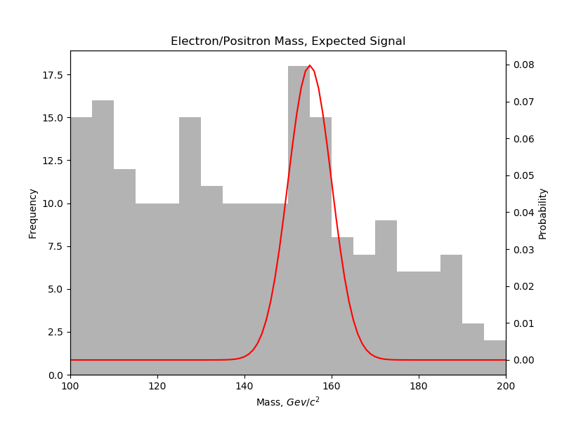
Extracting a signal from a sea of background noise? Look no further. We have simulated data of electron/positron pair production . We know that our signal mass is in the vicinity of 155 GeV, and we also know that our resolution is limited to ±5 Gev. Therefore our signal probability density function (PDF) is a Gaussian distribution with , . Our raw data and our expected signal can be seen in figure \ref{signal}. Now we want to fit a background PDF to filter how many signal versus background hits we actually measured.
Background PDF Selection
We have many options for our background PDF but by looking at our binned data we know we want something that is decreasing throughout the domain . Here I looked at 3 common families of distributions–the gamma distribution:
Where is the “shape parameter” and is the “scale parameter”. The function represents the gamma function. I also tried a log-normal distribution:
Where , follow the conventions of being the mean and standard deviation, but for the distribution pre-logarithm. Finally I looked at a simple, linear, monotonically decreasing distribution:
Where is the x-intercept of the distribution. These distributions cover a wide variety of potential PDF shapes. An exponential distribution is a subset of the gamma distribution so this choice of PDFs cover that possibility as well. The linear PDF was chosen not because I thought it would be particularly accurate, but more as a test to see how close such a simple, 1-parameter choice would be.
In all cases the PDFs are normalized as a function of their parameters on the interval by using the CDF at the endpoints:
However, there were issues with the gamma distribution not being normalized so instead I normalized it manually by summing over our list of points and then dividing each point by the total sum.
def gamma_norm( i, k, theta ):
    norm = []
    for n in x:
        norm.append( gamma_pdf( n, k, theta ) )
    return gamma_pdf( i, k, theta ) / math.fsum( norm )
This ensures that the points sum to 1 on our interval.
Optimizing Distributions
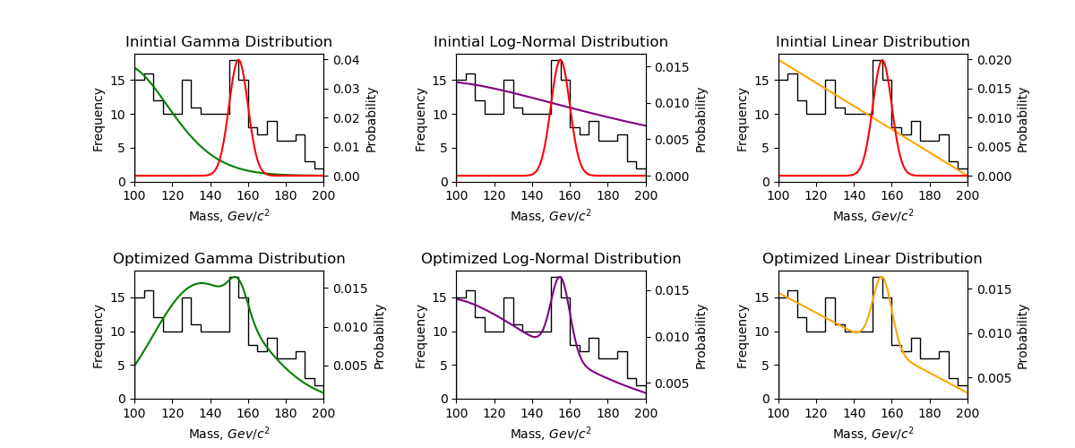 Top row is PDFs for initial parameter guesses. Bottom row is the PDFs
We now want to optimize the parameters of our PDFs to get closer to our measured values. We want to do this while separating our signal and background events so we can report the number of true signal hits. To do this we minimize a Negative Log Likelihood (NLL) fit:
Where , are the number of signal and background events, and , are the probability of the signal and background events at . Feeding this into Minuit to be minimized requires the addition of initial guesses for the of the parameters as well as step specification for the of all of the parameters. For all of the optimizations I initialized and as:
For the gamma, log-normal, and linear distributions I used:
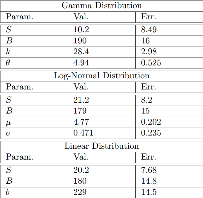
respectively. The step size was picked as either 1, 0.1, or 0.5 for most variables, except for which had a step size of 5 and for and which both had steps of 2. The PDFs for both the initial guesses and the optimized fits can be seen superimposed onto the data in figure \ref{pdf}, and the resulting optimized parameters can be seen in the table in figure 3.
Final Results
| Gamma Distribution |
| Param. | Val. | Err. |
|---|---|---|
| S | 10.2 | 8.5 |
| B | 190.0 | 16.0 |
| K | 28.4 | 3.0 |
| θ | 4.9 | 0.5 |
| Log-Normal Distribution |
| Parameter | Value | Error |
|---|---|---|
| S | 21.2 | 8.2 |
| B | 179.0 | 15.0 |
| μ | 4.8 | 0.2 |
| σ | 0.5 | 0.2 |
| Linear Distribution |
| Parameter | Value | Error |
|---|---|---|
| S | 20.2 | 7.7 |
| B | 180.0 | 14.8 |
| b | 229.0 | 14.5 |
The final parameters and error for the optimized gamma, log-normal, and linear distributions.
After optimization I was impressed by how well the linear PDF seemed to fit the data. I was equally as disappointed how poorly the gamma distribution fit. Since the gamma family covers a wide range of functions, including a decaying exponential, I expected that a minimization would be able to find some form that was a better fit. In fact, it seems to me that the shape of the “optimized” gamma PDF is actually farther from the data’s shape than the initial guess. Perhaps Minuit got stuck in a local minimum during it’s optimization. If there was more time I would like to continue playing with the gamma distribution. A different initial guess or a larger step size could potentially help it escape the minima it’s stuck in.
The linear and log-normal distribution were incredibly similar, with both reporting ~20 hits. I believe that the log-normal distribution matches the shape of the data slightly better, even though the linear fit technically achieved better accuracy (uncertainty of ±7.7 on the linear fit versus ±8.2 on the log fit). The background noise appears to be more constant at lower mass, which the log-normal fit captures better than the linear fit; it would require more data to see which fit truly excels.
The final log-normal background PDF is given by:
and results in:
where I took the floor of each number since it’s impossible to observe a partial event. The last uncertainty is taken from the standard deviation of the $S$ count from all three distributions. The standard deviation between $S_{gamma}, S_{log}, S_{lin}$ was $\sigma = 6.01$, but since two of the three distributions were in almost exact agreement with each other, I only took two-thirds of that error as my systematic uncertainty. An additional good sign is that the $S_{log}+B_{log} =200$ which is the correct number of total events, indicating our PDFs are properly normalized in relation to each other.
In Review
We tested the gamma, log-normal, and linear distributions against our data and each other to see which distribution best fit our data. The log-normal fit best, with the linear distribution fitting almost equally as well. The gamma distribution did surprisingly bad. Our final distribution was the normalized sum of our Gaussian and log-normal. This resulted in predicted signal events.
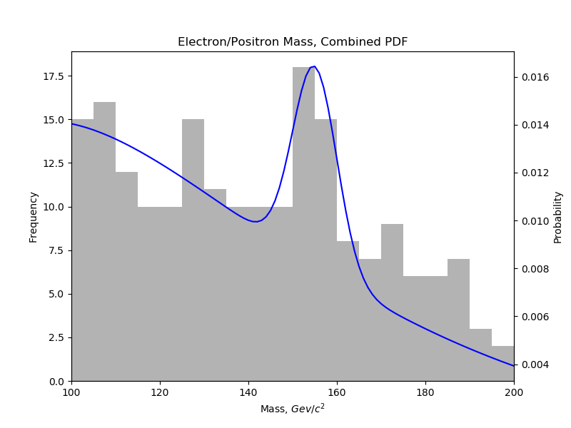 Final choice for the optimized PDF. The result was a log-normal distribution combined with our Gaussian signal. This predicts event results.